In the previous article, we described how we built a distributed least-request load balancer to spread requests evenly across GPU pods within a single Kubernetes cluster. That solved the local view problem and eliminated queueing. But we were still running on a single cloud provider.
GPU availability and pricing change constantly. Reserved instances run out, on-demand prices spike, new providers launch competitive offerings. Being locked into a single provider means you can’t take advantage of any of it. We needed a way to spread inference across multiple providers without rebuilding our stack for each one.
Kubernetes is cloud-agnostic by design, so we decided to lean into that: run identical inference clusters on multiple providers and build a layer to route traffic across them. The global load balancer is that layer.
The Setup
Currently we run on two Kubernetes clusters deployed on two different cloud providers (with plans to expand to more in the future). Each cluster runs the same stack: inference pods, Envoy proxies with our ext_proc-based local load balancer, and KEDA for autoscaling. One cluster has a pool of committed H100 GPUs. The other has both a committed pool and an on-demand pool of H100s.
The global load balancer sits in front of both clusters. When a request comes in for a given model, it picks which cluster should handle it based on weights derived from each cluster’s capacity. Inside the cluster, the local load balancer takes over and routes to the best pod.
Two layers, two concerns. The global LB decides where (which cluster), the local LB decides who (which pod).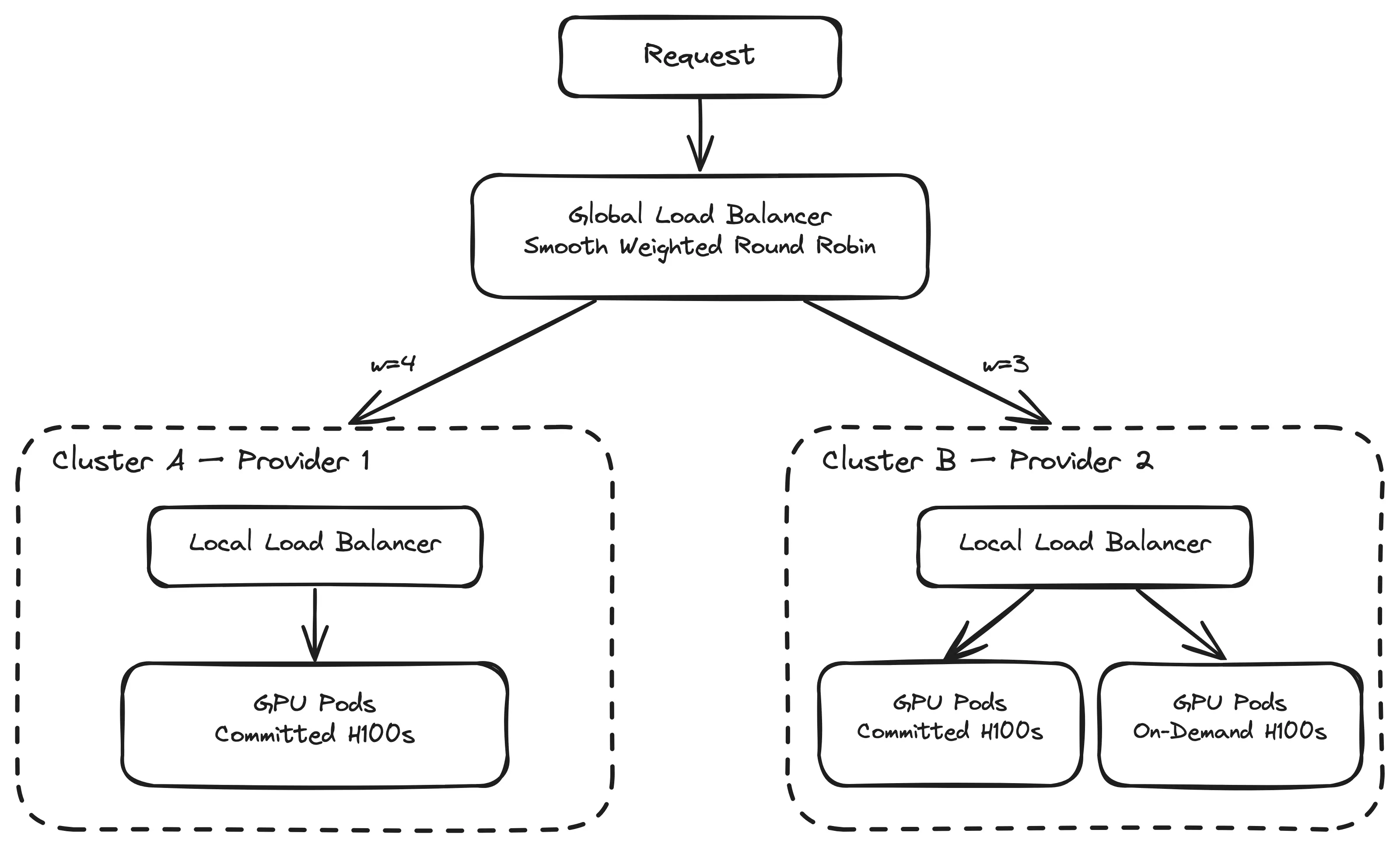 Multi provider architecture
Service Discovery: Knowing What’s Available
For the global LB to route requests, it needs to know two things: which clusters are running which models, and how much capacity each one has. We built a custom service discovery system for this, composed of two components: an endpoint watcher and a backend watcher.
Each cluster runs an endpoint watcher. It watches the Kubernetes API for EndpointSlices, counts how many pods are serving each model, and reports that count to the backend watcher.
The backend watcher receives these registrations from all clusters and computes weights. The logic is straightforward: for each model, it collects the capacity of every cluster serving it, computes the GCD of all capacities, and divides each capacity by the GCD to get normalized weights.
Here’s a concrete example with our two clusters serving the same model:
cluster-a:  8 pods
cluster-b:  6 pods

GCD(8, 6) = 2

cluster-a weight: 8 / 2 = 4
cluster-b weight: 6 / 2 = 3
Cluster A gets 4/7 of traffic (~57%), Cluster B gets 3/7 (~43%). The weights are proportional to capacity.
These weights are stored in a Redis sorted set. The global LB reads them on every request. When a cluster scales up or down, the endpoint watcher detects the change, re-registers with the backend watcher, weights are recomputed, and the global LB immediately routes according to the new distribution. No redeployment, no manual intervention.
If a cluster scales to zero pods for a model, its capacity drops to zero and it disappears from the weight set. When it scales back up, it reappears. The global LB doesn’t need to know about individual pods or node pools. It only cares about cluster-level capacity.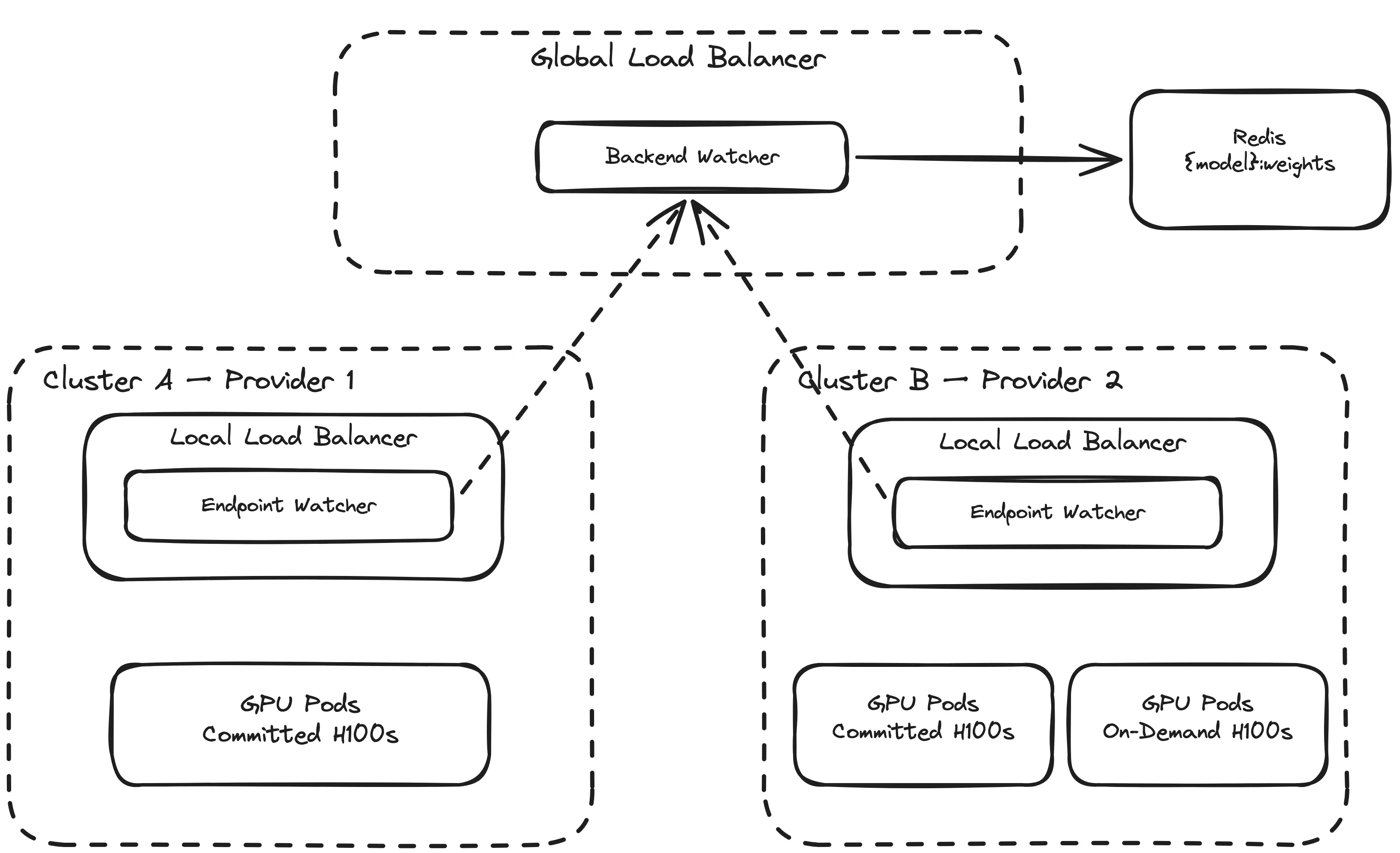
Routing: Smooth Weighted Round Robin
With weights in Redis, the global LB uses smooth weighted round robin to distribute traffic. This is a specific variant of weighted round robin that produces better interleaving than the naive approach.
The naive approach would be: with weights 4 and 3, send 4 requests to cluster A, then 3 to cluster B, then repeat. That creates bursts — AAAABBB AAAABBB — which means cluster B sits idle while cluster A handles its batch, and vice versa.
Smooth weighted round robin avoids this. The algorithm maintains a running counter (called “current weight”) for each cluster. On every request:
Add each cluster’s configured weight to its current weight
Select the cluster with the highest current weight
Subtract the total weight from the selected cluster’s current weight
Here’s what happens over 7 requests with weights A=4, B=3 (total=7):
Request  | Before add    | After add     | Selected | After subtract
---------|---------------|---------------|----------|---------------
1        | A=0,  B=0     | A=4,  B=3     | A        | A=-3, B=3
2        | A=-3, B=3     | A=1,  B=6     | B        | A=1,  B=-1
3        | A=1,  B=-1    | A=5,  B=2     | A        | A=-2, B=2
4        | A=-2, B=2     | A=2,  B=5     | B        | A=2,  B=-2
5        | A=2,  B=-2    | A=6,  B=1     | A        | A=-1, B=1
6        | A=-1, B=1     | A=3,  B=4     | B        | A=3,  B=-3
7        | A=-3, B=-3    | A=1,  B=0     | A        | A=-6, B=0
The pattern is A B A B A B A — perfectly interleaved. Over every 7 requests, A gets exactly 4 and B gets exactly 3, matching the 4:3 weight ratio. No bursts, no idle periods.
This matters because it keeps load smooth across clusters. Both clusters receive a steady stream of requests rather than alternating between busy and idle. Combined with the local load balancer distributing evenly across pods within each cluster, every GPU gets a consistent share of work.
When weights change — because a cluster scaled up, scaled down, or a new cluster was added — the algorithm detects the change and resets its internal state. The next request picks up the new weights immediately.
How It Fits Together
Here’s the full picture, from request to inference:
A request arrives at the global load balancer for model X
The global LB reads the weight sorted set for model X from Redis
Smooth weighted round robin selects a cluster (e.g., cluster-a)
The request is forwarded to cluster-a’s Envoy gateway
Envoy calls ext_proc, which queries the Redis sorted set for least-loaded pod
ext_proc returns the least-loaded pod’s IP
Envoy routes the request to that pod
The response flows back, decrementing the Redis counter
Steps 5–8 are the local load balancer from the previous article. Steps 1–4 are the global layer. The two are cleanly separated: the global LB has no visibility into individual pods, and the local LB has no awareness that other clusters exist.
Cost Optimization Through Local Scaling
One of the motivations for going multi-provider was cost. But the cost optimization doesn’t happen at the global LB level itself. It happens through consistent KEDA scaling policies across all clusters. KEDA is configured to scale pods onto committed nodes first — the cheapest capacity, already paid for — and only spills onto on-demand nodes when committed capacity is exhausted. The global LB doesn’t need to understand pricing or node types. It sends traffic proportionally to capacity, and each cluster handles its own cost efficiency internally.
Trade-offs
Service discovery is a new dependency. If the backend watcher is unavailable, the global LB can’t update its weights. We mitigate this by caching the last known good state in Redis. The weights persist until explicitly overwritten, so a temporary outage of the service discovery pipeline doesn’t disrupt routing. Stale weights are better than no weights.
Adding a new provider requires deploying the full stack. Kubernetes makes this manageable — the same manifests, same Helm charts, same configuration — but it’s still operational work. The payoff is that once a cluster is registered, the global LB picks it up automatically through service discovery.
Wrapping Up
The global load balancer is a thin layer with a narrow job: split traffic across clusters according to weights derived from their capacity. The complexity lives elsewhere — in the local load balancer for per-pod routing and in KEDA for cost-aware scaling.
The real value of this setup is flexibility. Adding a new GPU provider means spinning up a Kubernetes cluster, deploying the same stack, and letting service discovery propagate the weights. No changes to the routing logic, no new integrations. Kubernetes being cloud-agnostic makes this possible. The global LB makes it practical.
Between the local and global load balancers, we have a system that routes inference traffic evenly across pods, across clusters, and across providers. The local LB ensures no pod is overloaded. The global LB ensures we can take advantage of GPU capacity wherever it exists.